Kherson Dam Break end-to-end floodmap#
Last Modified: 30-11-2023
Authors: Gonzalo Mateo-García, Enrique Portalés-Julià
This notebook shows how to produce flood extent maps from Sentinel-2 and Landsat using the clouds aware flood sementation model proposed in:
E. Portalés-Julià, G. Mateo-García, C. Purcell, and L. Gómez-Chova Global flood extent segmentation in optical satellite images. Scientific Reports 13, 20316 (2023). DOI: 10.1038/s41598-023-47595-7.
In particular, the notebook shows how to: query the available S2 and Landsat images, download them, run inference with the model and vectorize the model outputs to derive prepost event floodmaps. We focus in the region of Nova Kakhovka, Kherson, Ukraine, where recently a dam break caused several flooding.
Note: If you run this notebook in Google Colab you may want to change the running environment to use a GPU.
Step 1: Install and import the necessary packages#
Install the ml4floods and geemap packages if not installed
!pip install geemap
!pip install ml4floods
import ee
# ee.Authenticate()
ee.Initialize()
from datetime import datetime, timezone
from georeader.readers import ee_query
from shapely.geometry import shape
import geopandas as gpd
from georeader.readers import S2_SAFE_reader
from georeader.save import save_cog
from georeader import window_utils, mosaic
from georeader import plot
from georeader.rasterio_reader import RasterioReader
import os
import torch
import numpy as np
from georeader.geotensor import GeoTensor
from ml4floods.scripts.inference import load_inference_function, vectorize_outputv1
from ml4floods.models.model_setup import get_channel_configuration_bands
from ml4floods.data import utils
import warnings
from georeader.readers import ee_image
from ml4floods.models import postprocess
from georeader import plot
import matplotlib.pyplot as plt
from ml4floods.visualization import plot_utils
Step 2: Define query parameters: area of interest and dates#
The area of interest covers the region from Nova Kakhovka to Kherson. The following code defines this AoI and queries the available S2 and Landsat images and shows them using geemap.
aoi = shape({'type': 'Polygon',
 'coordinates': (((33.40965055141422, 46.849975215311474),
   (33.24671826582107, 46.923511440491325),
   (32.936224664974134, 46.845770100334164),
   (32.33368262768653, 46.62876156455022),
   (32.25990197005967, 46.514641087646424),
   (32.31216326921171, 46.408759851523826),
   (32.843998842939385, 46.56961795883814),
   (33.21905051921081, 46.72367854887557),
   (33.40965055141422, 46.849975215311474)),)})

aoi_gpd = gpd.GeoDataFrame({'geometry':aoi},index = [0]).set_crs('epsg:4326')
Step 3: Query available Landsat and Sentinel-2 images#
tz = timezone.utc
start_period = datetime.strptime('2023-05-31',"%Y-%m-%d").replace(tzinfo=tz)
end_period = datetime.strptime('2023-06-12',"%Y-%m-%d").replace(tzinfo=tz)

# This function returns a GEE collection of Sentinel-2 and Landsat 8 data and a Geopandas Dataframe with data related to the tiles, overlap percentage and cloud cover
flood_images_gee, flood_collection = ee_query.query(
    area=aoi,
    date_start=start_period,
    date_end=end_period,
    producttype="both",
    return_collection=True,
    add_s2cloudless=False)

flood_images_gee.groupby(["solarday","satellite"])[["cloudcoverpercentage","overlappercentage"]].agg(["count","mean"])
| cloudcoverpercentage | overlappercentage | ||||
|---|---|---|---|---|---|
| count | mean | count | mean | ||
| solarday | satellite | ||||
| 2023-05-31 | S2B | 2 | 75.062169 | 2 | 27.434830 |
| 2023-06-01 | LC08 | 2 | 2.070000 | 2 | 78.634958 |
| 2023-06-02 | LC09 | 1 | 16.040000 | 1 | 75.542523 |
| 2023-06-03 | S2B | 2 | 4.788626 | 2 | 56.100742 |
| 2023-06-05 | S2A | 2 | 0.000000 | 2 | 27.990063 |
| 2023-06-08 | S2A | 2 | 95.540035 | 2 | 56.100742 |
| 2023-06-09 | LC09 | 2 | 7.760000 | 2 | 79.054185 |
| 2023-06-10 | LC08 | 1 | 93.430000 | 1 | 67.152296 |
| S2B | 2 | 99.942521 | 2 | 27.707824 | |
import geemap.foliumap as geemap
import folium

tl = folium.TileLayer(
            tiles="https://mt1.google.com/vt/lyrs=s&x={x}&y={y}&z={z}",
            attr='Google',
            name="Google Satellite",
            overlay=True,
            control=True,
            max_zoom=22,
        )

m = geemap.Map(location=aoi.centroid.coords[0][-1::-1],
               zoom_start=8)

tl.add_to(m)

flood_images_gee["localdatetime_str"] = flood_images_gee["localdatetime"].dt.strftime("%Y-%m-%d %H:%M:%S")
showcolumns = ["geometry","overlappercentage","cloudcoverpercentage", "localdatetime_str","solarday","satellite"]
colors = ["#ff7777", "#fffa69", "#8fff84", "#52adf1", "#ff6ac2","#1b6d52", "#fce5cd","#705334"]

# Add the extent of the products
for i, ((day,satellite), images_day) in enumerate(flood_images_gee.groupby(["solarday","satellite"])):
    images_day[showcolumns].explore(
        m=m,
        name=f"{satellite}: {day} outline",
        color=colors[i % len(colors)],
        show=False)

# Add the satellite data
for (day, satellite), images_day in flood_images_gee.groupby(["solarday", "satellite"]):
    image_col_day_sat = flood_collection.filter(ee.Filter.inList("title", images_day.index.tolist()))
    bands = ["B11","B8","B4"] if satellite.startswith("S2") else ["B6","B5","B4"]
    m.addLayer(image_col_day_sat,
               {"min":0, "max":3000 if satellite.startswith("S2") else 0.3, "bands": bands},
               f"{satellite}: {day}",
               False)

aoi_gpd.explore(style_kwds={"fillOpacity": 0}, color="black", name="AoI", m=m)
folium.LayerControl(collapsed=False).add_to(m)
m
By looking at the map with the images available we select the pre and post event images from Sentinel-2
date_pre = "2023-06-03"
pre_flood = flood_images_gee[flood_images_gee.solarday == date_pre]

date_post = "2023-06-08"
post_flood = flood_images_gee[flood_images_gee.solarday == date_post]
post_flood
| geometry | cloudcoverpercentage | gee_id | proj | system:time_start | collection_name | utcdatetime | overlappercentage | solardatetime | solarday | localdatetime | satellite | localdatetime_str | |
|---|---|---|---|---|---|---|---|---|---|---|---|---|---|
| title | |||||||||||||
| S2A_MSIL1C_20230608T084601_N0509_R107_T36TVS_20230608T104959 | POLYGON ((31.70898 45.95835, 31.709 45.95835, ... | 91.090149 | 20230608T084601_20230608T084938_T36TVS | {'type': 'Projection', 'crs': 'EPSG:32636', 't... | 1686214645530 | COPERNICUS/S2_HARMONIZED | 2023-06-08 08:57:25.530000+00:00 | 83.282631 | 2023-06-08 11:07:04.427835+00:00 | 2023-06-08 | 2023-06-08 08:57:25.530000+00:00 | S2A | 2023-06-08 08:57:25 |
| S2A_MSIL1C_20230608T084601_N0509_R107_T36TWS_20230608T104959 | POLYGON ((34.44238 46.94462, 34.44228 46.94471... | 99.989920 | 20230608T084601_20230608T084938_T36TWS | {'type': 'Projection', 'crs': 'EPSG:32636', 't... | 1686214640951 | COPERNICUS/S2_HARMONIZED | 2023-06-08 08:57:20.951000+00:00 | 28.918853 | 2023-06-08 11:11:50.363462+00:00 | 2023-06-08 | 2023-06-08 08:57:20.951000+00:00 | S2A | 2023-06-08 08:57:20 |
Step 4: Download Sentinel-2 images#
There are Sentinel-2 cloud free images on 2023-06-03 and 2023-06-05 but only the first one covers the entire AoI. For the postflood data we will use 2023-06-08, which is partially cloudy but allows to see some flood extent. We will read and mosaic the tiles T36TVS and T36TWS using georeader. The advantage of this workflow over Google Earth Engine (GEE) is that the images are read directly from the Sentinel-2 public bucket into the jupyter notebook. Also, there is no size limit in the download, which may cause GEE tasks to fail sometimes.
%%time
from shapely.geometry import Polygon, MultiPolygon


def mosaic_s2(products, polygon, channels):
    s2objs = []

    # Old code reading from S2 public bucket
    # products_read = products.index
    # for product in products_read:
    #     s2_safe_folder = S2_SAFE_reader.s2_public_bucket_path(product+".SAFE", check_exists=False)
    #     s2obj = S2_SAFE_reader.s2loader(s2_safe_folder, out_res=10, bands=channels)
    #     s2obj = s2obj.cache_product_to_local_dir(dir_cache)
    #     s2objs.append(s2obj)

    # Query from the GEE
    channels_query = [c.replace("B0","B") for c in channels]
    for d in products.itertuples():
        asset_id = f"{d.collection_name}/{d.gee_id}"
        geom = d.geometry.intersection(polygon)
        if not isinstance(geom, (Polygon, MultiPolygon)):
            print(f"Weird geometry: {geom} we will skip it")
            continue

        data_geotensor = ee_image.export_image_getpixels(asset_id, geom, proj=d.proj,
                                                         bands_gee=channels_query)
        s2objs.append(data_geotensor)

    # Mosaic the rasters
    polygon_read_dst_crs = window_utils.polygon_to_crs(polygon,
                                                       crs_polygon="EPSG:4326", dst_crs=s2objs[0].crs)

    data_memory = mosaic.spatial_mosaic(s2objs, polygon=polygon_read_dst_crs, dst_crs= s2objs[0].crs)

    return data_memory

channels = S2_SAFE_reader.BANDS_S2_L1C
tiff_pre = f"{date_pre}.tif"
if not os.path.exists(tiff_pre):
    print(f"Downloading files {tiff_pre}")
    pre_flood_memory = mosaic_s2(pre_flood, aoi,channels)
    pre_flood = pre_flood_memory
    save_cog(pre_flood_memory, tiff_pre, descriptions=S2_SAFE_reader.BANDS_S2_L1C)
else:
    print(f"Reading file {tiff_pre}")
    pre_flood = RasterioReader(tiff_pre)
    channels = pre_flood.descriptions
    pre_flood_memory = pre_flood

tiff_post = f"{date_post}.tif"
if not os.path.exists(tiff_post):
    print(f"Downloading file {tiff_post}")
    post_flood_memory = mosaic_s2(post_flood, aoi,channels)
    post_flood = post_flood_memory
    save_cog(post_flood_memory, tiff_post, descriptions=S2_SAFE_reader.BANDS_S2_L1C)
else:
    print(f"Reading file {tiff_post}")
    post_flood = RasterioReader(tiff_post)
    channels = post_flood.descriptions
    post_flood_memory = post_flood.load()
Downloading files 2023-06-03.tif
/home/gonzalo/git/georeader/georeader/readers/ee_image.py:152: UserWarning: Geometry POINT (32.54506832764637 46.70489318424674) is not a Polygon or MultiPolygon, skipping it.
  warnings.warn(
Warning 1: TIFFReadDirectory:Sum of Photometric type-related color channels and ExtraSamples doesn't match SamplesPerPixel. Defining non-color channels as ExtraSamples.
Warning 1: TIFFReadDirectory:Sum of Photometric type-related color channels and ExtraSamples doesn't match SamplesPerPixel. Defining non-color channels as ExtraSamples.
Warning 1: TIFFReadDirectory:Sum of Photometric type-related color channels and ExtraSamples doesn't match SamplesPerPixel. Defining non-color channels as ExtraSamples.
Warning 1: TIFFReadDirectory:Sum of Photometric type-related color channels and ExtraSamples doesn't match SamplesPerPixel. Defining non-color channels as ExtraSamples.
Warning 1: TIFFReadDirectory:Sum of Photometric type-related color channels and ExtraSamples doesn't match SamplesPerPixel. Defining non-color channels as ExtraSamples.
Warning 1: TIFFReadDirectory:Sum of Photometric type-related color channels and ExtraSamples doesn't match SamplesPerPixel. Defining non-color channels as ExtraSamples.
Warning 1: TIFFReadDirectory:Sum of Photometric type-related color channels and ExtraSamples doesn't match SamplesPerPixel. Defining non-color channels as ExtraSamples.
Warning 1: TIFFReadDirectory:Sum of Photometric type-related color channels and ExtraSamples doesn't match SamplesPerPixel. Defining non-color channels as ExtraSamples.
Warning 1: TIFFReadDirectory:Sum of Photometric type-related color channels and ExtraSamples doesn't match SamplesPerPixel. Defining non-color channels as ExtraSamples.
Warning 1: TIFFReadDirectory:Sum of Photometric type-related color channels and ExtraSamples doesn't match SamplesPerPixel. Defining non-color channels as ExtraSamples.
Warning 1: TIFFReadDirectory:Sum of Photometric type-related color channels and ExtraSamples doesn't match SamplesPerPixel. Defining non-color channels as ExtraSamples.
Warning 1: TIFFReadDirectory:Sum of Photometric type-related color channels and ExtraSamples doesn't match SamplesPerPixel. Defining non-color channels as ExtraSamples.
Warning 1: TIFFReadDirectory:Sum of Photometric type-related color channels and ExtraSamples doesn't match SamplesPerPixel. Defining non-color channels as ExtraSamples.
Warning 1: TIFFReadDirectory:Sum of Photometric type-related color channels and ExtraSamples doesn't match SamplesPerPixel. Defining non-color channels as ExtraSamples.
Warning 1: TIFFReadDirectory:Sum of Photometric type-related color channels and ExtraSamples doesn't match SamplesPerPixel. Defining non-color channels as ExtraSamples.
Warning 1: TIFFReadDirectory:Sum of Photometric type-related color channels and ExtraSamples doesn't match SamplesPerPixel. Defining non-color channels as ExtraSamples.
Warning 1: TIFFReadDirectory:Sum of Photometric type-related color channels and ExtraSamples doesn't match SamplesPerPixel. Defining non-color channels as ExtraSamples.
Warning 1: TIFFReadDirectory:Sum of Photometric type-related color channels and ExtraSamples doesn't match SamplesPerPixel. Defining non-color channels as ExtraSamples.
Warning 1: TIFFReadDirectory:Sum of Photometric type-related color channels and ExtraSamples doesn't match SamplesPerPixel. Defining non-color channels as ExtraSamples.
Warning 1: TIFFReadDirectory:Sum of Photometric type-related color channels and ExtraSamples doesn't match SamplesPerPixel. Defining non-color channels as ExtraSamples.
Warning 1: TIFFReadDirectory:Sum of Photometric type-related color channels and ExtraSamples doesn't match SamplesPerPixel. Defining non-color channels as ExtraSamples.
Warning 1: TIFFReadDirectory:Sum of Photometric type-related color channels and ExtraSamples doesn't match SamplesPerPixel. Defining non-color channels as ExtraSamples.
Warning 1: TIFFReadDirectory:Sum of Photometric type-related color channels and ExtraSamples doesn't match SamplesPerPixel. Defining non-color channels as ExtraSamples.
Warning 1: TIFFReadDirectory:Sum of Photometric type-related color channels and ExtraSamples doesn't match SamplesPerPixel. Defining non-color channels as ExtraSamples.
Warning 1: TIFFReadDirectory:Sum of Photometric type-related color channels and ExtraSamples doesn't match SamplesPerPixel. Defining non-color channels as ExtraSamples.
Warning 1: TIFFReadDirectory:Sum of Photometric type-related color channels and ExtraSamples doesn't match SamplesPerPixel. Defining non-color channels as ExtraSamples.
Warning 1: TIFFReadDirectory:Sum of Photometric type-related color channels and ExtraSamples doesn't match SamplesPerPixel. Defining non-color channels as ExtraSamples.
Warning 1: TIFFReadDirectory:Sum of Photometric type-related color channels and ExtraSamples doesn't match SamplesPerPixel. Defining non-color channels as ExtraSamples.
Warning 1: TIFFReadDirectory:Sum of Photometric type-related color channels and ExtraSamples doesn't match SamplesPerPixel. Defining non-color channels as ExtraSamples.
Warning 1: TIFFReadDirectory:Sum of Photometric type-related color channels and ExtraSamples doesn't match SamplesPerPixel. Defining non-color channels as ExtraSamples.
Warning 1: TIFFReadDirectory:Sum of Photometric type-related color channels and ExtraSamples doesn't match SamplesPerPixel. Defining non-color channels as ExtraSamples.
Warning 1: TIFFReadDirectory:Sum of Photometric type-related color channels and ExtraSamples doesn't match SamplesPerPixel. Defining non-color channels as ExtraSamples.
Warning 1: TIFFReadDirectory:Sum of Photometric type-related color channels and ExtraSamples doesn't match SamplesPerPixel. Defining non-color channels as ExtraSamples.
Warning 1: TIFFReadDirectory:Sum of Photometric type-related color channels and ExtraSamples doesn't match SamplesPerPixel. Defining non-color channels as ExtraSamples.
Warning 1: TIFFReadDirectory:Sum of Photometric type-related color channels and ExtraSamples doesn't match SamplesPerPixel. Defining non-color channels as ExtraSamples.
Warning 1: TIFFReadDirectory:Sum of Photometric type-related color channels and ExtraSamples doesn't match SamplesPerPixel. Defining non-color channels as ExtraSamples.
Warning 1: TIFFReadDirectory:Sum of Photometric type-related color channels and ExtraSamples doesn't match SamplesPerPixel. Defining non-color channels as ExtraSamples.
Warning 1: TIFFReadDirectory:Sum of Photometric type-related color channels and ExtraSamples doesn't match SamplesPerPixel. Defining non-color channels as ExtraSamples.
Warning 1: TIFFReadDirectory:Sum of Photometric type-related color channels and ExtraSamples doesn't match SamplesPerPixel. Defining non-color channels as ExtraSamples.
Warning 1: TIFFReadDirectory:Sum of Photometric type-related color channels and ExtraSamples doesn't match SamplesPerPixel. Defining non-color channels as ExtraSamples.
Warning 1: TIFFReadDirectory:Sum of Photometric type-related color channels and ExtraSamples doesn't match SamplesPerPixel. Defining non-color channels as ExtraSamples.
Warning 1: TIFFReadDirectory:Sum of Photometric type-related color channels and ExtraSamples doesn't match SamplesPerPixel. Defining non-color channels as ExtraSamples.
Warning 1: TIFFReadDirectory:Sum of Photometric type-related color channels and ExtraSamples doesn't match SamplesPerPixel. Defining non-color channels as ExtraSamples.
Warning 1: TIFFReadDirectory:Sum of Photometric type-related color channels and ExtraSamples doesn't match SamplesPerPixel. Defining non-color channels as ExtraSamples.
Warning 1: TIFFReadDirectory:Sum of Photometric type-related color channels and ExtraSamples doesn't match SamplesPerPixel. Defining non-color channels as ExtraSamples.
Warning 1: TIFFReadDirectory:Sum of Photometric type-related color channels and ExtraSamples doesn't match SamplesPerPixel. Defining non-color channels as ExtraSamples.
Warning 1: TIFFReadDirectory:Sum of Photometric type-related color channels and ExtraSamples doesn't match SamplesPerPixel. Defining non-color channels as ExtraSamples.
Warning 1: TIFFReadDirectory:Sum of Photometric type-related color channels and ExtraSamples doesn't match SamplesPerPixel. Defining non-color channels as ExtraSamples.
Warning 1: TIFFReadDirectory:Sum of Photometric type-related color channels and ExtraSamples doesn't match SamplesPerPixel. Defining non-color channels as ExtraSamples.
Downloading file 2023-06-08.tif
Warning 1: TIFFReadDirectory:Sum of Photometric type-related color channels and ExtraSamples doesn't match SamplesPerPixel. Defining non-color channels as ExtraSamples.
Warning 1: TIFFReadDirectory:Sum of Photometric type-related color channels and ExtraSamples doesn't match SamplesPerPixel. Defining non-color channels as ExtraSamples.
Warning 1: TIFFReadDirectory:Sum of Photometric type-related color channels and ExtraSamples doesn't match SamplesPerPixel. Defining non-color channels as ExtraSamples.
Warning 1: TIFFReadDirectory:Sum of Photometric type-related color channels and ExtraSamples doesn't match SamplesPerPixel. Defining non-color channels as ExtraSamples.
Warning 1: TIFFReadDirectory:Sum of Photometric type-related color channels and ExtraSamples doesn't match SamplesPerPixel. Defining non-color channels as ExtraSamples.
Warning 1: TIFFReadDirectory:Sum of Photometric type-related color channels and ExtraSamples doesn't match SamplesPerPixel. Defining non-color channels as ExtraSamples.
Warning 1: TIFFReadDirectory:Sum of Photometric type-related color channels and ExtraSamples doesn't match SamplesPerPixel. Defining non-color channels as ExtraSamples.
Warning 1: TIFFReadDirectory:Sum of Photometric type-related color channels and ExtraSamples doesn't match SamplesPerPixel. Defining non-color channels as ExtraSamples.
Warning 1: TIFFReadDirectory:Sum of Photometric type-related color channels and ExtraSamples doesn't match SamplesPerPixel. Defining non-color channels as ExtraSamples.
Warning 1: TIFFReadDirectory:Sum of Photometric type-related color channels and ExtraSamples doesn't match SamplesPerPixel. Defining non-color channels as ExtraSamples.
Warning 1: TIFFReadDirectory:Sum of Photometric type-related color channels and ExtraSamples doesn't match SamplesPerPixel. Defining non-color channels as ExtraSamples.
Warning 1: TIFFReadDirectory:Sum of Photometric type-related color channels and ExtraSamples doesn't match SamplesPerPixel. Defining non-color channels as ExtraSamples.
Warning 1: TIFFReadDirectory:Sum of Photometric type-related color channels and ExtraSamples doesn't match SamplesPerPixel. Defining non-color channels as ExtraSamples.
Warning 1: TIFFReadDirectory:Sum of Photometric type-related color channels and ExtraSamples doesn't match SamplesPerPixel. Defining non-color channels as ExtraSamples.
Warning 1: TIFFReadDirectory:Sum of Photometric type-related color channels and ExtraSamples doesn't match SamplesPerPixel. Defining non-color channels as ExtraSamples.
Warning 1: TIFFReadDirectory:Sum of Photometric type-related color channels and ExtraSamples doesn't match SamplesPerPixel. Defining non-color channels as ExtraSamples.
Warning 1: TIFFReadDirectory:Sum of Photometric type-related color channels and ExtraSamples doesn't match SamplesPerPixel. Defining non-color channels as ExtraSamples.
Warning 1: TIFFReadDirectory:Sum of Photometric type-related color channels and ExtraSamples doesn't match SamplesPerPixel. Defining non-color channels as ExtraSamples.
Warning 1: TIFFReadDirectory:Sum of Photometric type-related color channels and ExtraSamples doesn't match SamplesPerPixel. Defining non-color channels as ExtraSamples.
Warning 1: TIFFReadDirectory:Sum of Photometric type-related color channels and ExtraSamples doesn't match SamplesPerPixel. Defining non-color channels as ExtraSamples.
Warning 1: TIFFReadDirectory:Sum of Photometric type-related color channels and ExtraSamples doesn't match SamplesPerPixel. Defining non-color channels as ExtraSamples.
Warning 1: TIFFReadDirectory:Sum of Photometric type-related color channels and ExtraSamples doesn't match SamplesPerPixel. Defining non-color channels as ExtraSamples.
Warning 1: TIFFReadDirectory:Sum of Photometric type-related color channels and ExtraSamples doesn't match SamplesPerPixel. Defining non-color channels as ExtraSamples.
Warning 1: TIFFReadDirectory:Sum of Photometric type-related color channels and ExtraSamples doesn't match SamplesPerPixel. Defining non-color channels as ExtraSamples.
Warning 1: TIFFReadDirectory:Sum of Photometric type-related color channels and ExtraSamples doesn't match SamplesPerPixel. Defining non-color channels as ExtraSamples.
Warning 1: TIFFReadDirectory:Sum of Photometric type-related color channels and ExtraSamples doesn't match SamplesPerPixel. Defining non-color channels as ExtraSamples.
Warning 1: TIFFReadDirectory:Sum of Photometric type-related color channels and ExtraSamples doesn't match SamplesPerPixel. Defining non-color channels as ExtraSamples.
Warning 1: TIFFReadDirectory:Sum of Photometric type-related color channels and ExtraSamples doesn't match SamplesPerPixel. Defining non-color channels as ExtraSamples.
Warning 1: TIFFReadDirectory:Sum of Photometric type-related color channels and ExtraSamples doesn't match SamplesPerPixel. Defining non-color channels as ExtraSamples.
Warning 1: TIFFReadDirectory:Sum of Photometric type-related color channels and ExtraSamples doesn't match SamplesPerPixel. Defining non-color channels as ExtraSamples.
Warning 1: TIFFReadDirectory:Sum of Photometric type-related color channels and ExtraSamples doesn't match SamplesPerPixel. Defining non-color channels as ExtraSamples.
Warning 1: TIFFReadDirectory:Sum of Photometric type-related color channels and ExtraSamples doesn't match SamplesPerPixel. Defining non-color channels as ExtraSamples.
Warning 1: TIFFReadDirectory:Sum of Photometric type-related color channels and ExtraSamples doesn't match SamplesPerPixel. Defining non-color channels as ExtraSamples.
Warning 1: TIFFReadDirectory:Sum of Photometric type-related color channels and ExtraSamples doesn't match SamplesPerPixel. Defining non-color channels as ExtraSamples.
Warning 1: TIFFReadDirectory:Sum of Photometric type-related color channels and ExtraSamples doesn't match SamplesPerPixel. Defining non-color channels as ExtraSamples.
Warning 1: TIFFReadDirectory:Sum of Photometric type-related color channels and ExtraSamples doesn't match SamplesPerPixel. Defining non-color channels as ExtraSamples.
Warning 1: TIFFReadDirectory:Sum of Photometric type-related color channels and ExtraSamples doesn't match SamplesPerPixel. Defining non-color channels as ExtraSamples.
Warning 1: TIFFReadDirectory:Sum of Photometric type-related color channels and ExtraSamples doesn't match SamplesPerPixel. Defining non-color channels as ExtraSamples.
Warning 1: TIFFReadDirectory:Sum of Photometric type-related color channels and ExtraSamples doesn't match SamplesPerPixel. Defining non-color channels as ExtraSamples.
Warning 1: TIFFReadDirectory:Sum of Photometric type-related color channels and ExtraSamples doesn't match SamplesPerPixel. Defining non-color channels as ExtraSamples.
Warning 1: TIFFReadDirectory:Sum of Photometric type-related color channels and ExtraSamples doesn't match SamplesPerPixel. Defining non-color channels as ExtraSamples.
Warning 1: TIFFReadDirectory:Sum of Photometric type-related color channels and ExtraSamples doesn't match SamplesPerPixel. Defining non-color channels as ExtraSamples.
Warning 1: TIFFReadDirectory:Sum of Photometric type-related color channels and ExtraSamples doesn't match SamplesPerPixel. Defining non-color channels as ExtraSamples.
Warning 1: TIFFReadDirectory:Sum of Photometric type-related color channels and ExtraSamples doesn't match SamplesPerPixel. Defining non-color channels as ExtraSamples.
Warning 1: TIFFReadDirectory:Sum of Photometric type-related color channels and ExtraSamples doesn't match SamplesPerPixel. Defining non-color channels as ExtraSamples.
Warning 1: TIFFReadDirectory:Sum of Photometric type-related color channels and ExtraSamples doesn't match SamplesPerPixel. Defining non-color channels as ExtraSamples.
Warning 1: TIFFReadDirectory:Sum of Photometric type-related color channels and ExtraSamples doesn't match SamplesPerPixel. Defining non-color channels as ExtraSamples.
Warning 1: TIFFReadDirectory:Sum of Photometric type-related color channels and ExtraSamples doesn't match SamplesPerPixel. Defining non-color channels as ExtraSamples.
Warning 1: TIFFReadDirectory:Sum of Photometric type-related color channels and ExtraSamples doesn't match SamplesPerPixel. Defining non-color channels as ExtraSamples.
CPU times: user 4min 27s, sys: 21.6 s, total: 4min 49s
Wall time: 4min 57s
Step 5: Load the model#
For this we will use an Ml4floods multioutput binary model trained on the WorldFloods data set. See the paper.
from huggingface_hub import hf_hub_download
# os.makedirs("models/WF2_unetv2_bgriswirs", exist_ok=True)
experiment_name = "WF2_unetv2_bgriswirs"
subfolder_local = f"models/{experiment_name}"
config_file = hf_hub_download(repo_id="isp-uv-es/ml4floods",subfolder=subfolder_local, filename="config.json",
                              local_dir=".", local_dir_use_symlinks=False)
model_file = hf_hub_download(repo_id="isp-uv-es/ml4floods",subfolder=subfolder_local, filename="model.pt",
                              local_dir=".", local_dir_use_symlinks=False)
%%time

inference_function, config = load_inference_function(subfolder_local, device_name = 'cpu', max_tile_size=1024,
                                                     th_water=0.6, th_brightness=3500,
                                                     distinguish_flood_traces=True)

channel_configuration = config['data_params']['channel_configuration']
channels_inference  = get_channel_configuration_bands(channel_configuration, collection_name='S2')
Loaded model weights: models/WF2_unetv2_bgriswirs/model.pt
Getting model inference function
CPU times: user 294 ms, sys: 14.8 ms, total: 309 ms
Wall time: 208 ms
def predict(input_tensor, channels = [1, 2, 3, 7, 11, 12] ):
    input_tensor = input_tensor.astype(np.float32)
    input_tensor = input_tensor[channels]
    torch_inputs = torch.tensor(np.nan_to_num(input_tensor))
    return inference_function(torch_inputs)
Step 6: Run inference on Sentinel-2 images#
%%time

postflood_pred = f"{date_post}_pred.tif"
if not os.path.exists(postflood_pred):
    print("Computing post-flood prediction")
    prediction_postflood, prediction_postflood_cont  = predict(post_flood_memory.values)
    prediction_postflood_raster = GeoTensor(prediction_postflood.numpy(),
                                            transform=post_flood_memory.transform,
                                            fill_value_default=0, crs=post_flood_memory.crs)
    save_cog(prediction_postflood_raster, postflood_pred, descriptions=["pred"],
             tags={"0":"invalid", "1": "land", "2":"water", "3":"cloud", "4":"flood_trace"})
else:
    prediction_postflood_raster = RasterioReader(postflood_pred).load().squeeze()

preflood_pred = f"{date_pre}_pred.tif"
if not os.path.exists(preflood_pred):
    print("Computing pre-flood prediction")
    prediction_preflood, prediction_preflood_cont = predict(pre_flood_memory.values)
    # Remove flood traces from pre-flood
    prediction_preflood[prediction_preflood==4] = 1

    prediction_preflood_raster = GeoTensor(prediction_preflood.numpy(), transform=pre_flood_memory.transform,
                                           fill_value_default=0, crs=pre_flood_memory.crs)

    save_cog(prediction_preflood_raster, preflood_pred, descriptions=["pred"],
             tags={"0":"invalid", "1": "land", "2":"water", "3":"cloud", "4":"flood_trace"})
else:
    prediction_preflood_raster = RasterioReader(preflood_pred).load().squeeze()
Computing post-flood prediction
Computing pre-flood prediction
CPU times: user 1h 33min 10s, sys: 12min 31s, total: 1h 45min 41s
Wall time: 14min 11s
COLORS_PRED = np.array([[0, 0, 0], # 0: invalid
                       [139, 64, 0], # 1: land
                       [0, 0, 240], # 2: water
                       [220, 220, 220], # 3: cloud
                       [60, 85, 92]], # 5: flood_trace
                    dtype=np.float32) / 255
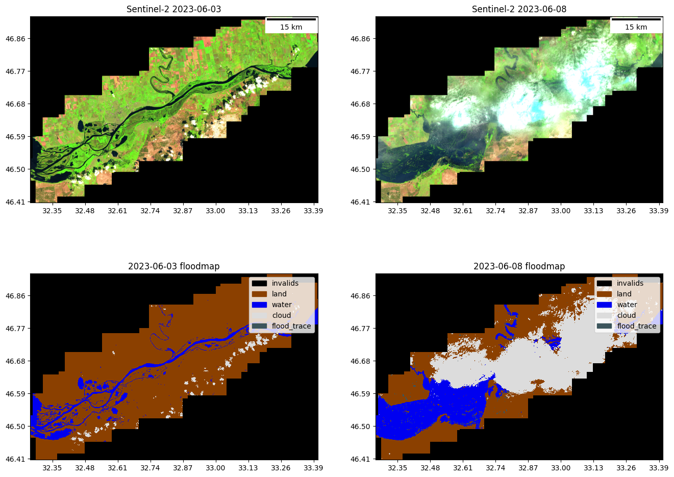
Step 7: Plot Sentinel-2 images and floodmaps#
fig, ax = plt.subplots(2,2,figsize=(16,12),squeeze=False)

swirnirred_idx = [channels.index(b) for b in ["B11", "B08", "B04"]]
swir_nirred_pre = (pre_flood_memory.isel({"band": swirnirred_idx}) / 3500).clip(0, 1)

plot.show(swir_nirred_pre, ax = ax[0,0], add_scalebar = True, title=f"Sentinel-2 {date_pre}")

swir_nirred_post = (post_flood_memory.isel({"band":swirnirred_idx}) / 3500).clip(0, 1)

plot.show(swir_nirred_post,ax = ax[0,1], add_scalebar = True,
     title=f"Sentinel-2 {date_post}")

plot.plot_segmentation_mask(prediction_preflood_raster, COLORS_PRED, ax=ax[1,0],
                            interpretation_array=["invalids", "land", "water", "cloud", "flood_trace"])

ax[1,0].set_title(f"{date_pre} floodmap")

plot.plot_segmentation_mask(prediction_postflood_raster, COLORS_PRED, ax=ax[1,1],
                            interpretation_array=["invalids", "land", "water", "cloud", "flood_trace"])

ax[1,1].set_title(f"{date_post} floodmap")
Text(0.5, 1.0, '2023-06-08 floodmap')
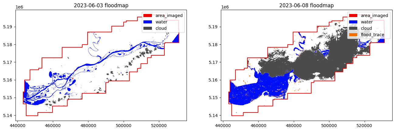
Step 8: Vectorize predictions into prepost flood products#
preflood_shape = vectorize_outputv1(prediction_preflood_raster.values,
                                    prediction_preflood_raster.crs,
                                    prediction_preflood_raster.transform)
postflood_shape = vectorize_outputv1(prediction_postflood_raster.values,
                                     prediction_postflood_raster.crs,
                                     prediction_postflood_raster.transform)
postflood_shape.shape
(1786, 3)
fig, ax = plt.subplots(1, 2, figsize=(16, 12))
plot_utils.plot_floodmap(preflood_shape, ax=ax[0])
ax[0].set_title(f"{date_pre} floodmap")
plot_utils.plot_floodmap(postflood_shape, ax=ax[1])
ax[1].set_title(f"{date_post} floodmap")
Text(0.5, 1.0, '2023-06-08 floodmap')
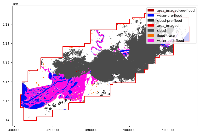
prepost_shape = postprocess.compute_pre_post_flood_water(postflood_shape, preflood_shape)
plot_utils.plot_floodmap(prepost_shape)
<Axes: >
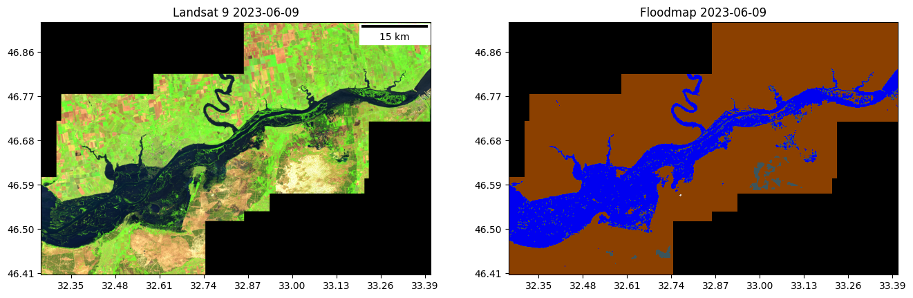
Step 9: Download Landsat 8/9#
There is a cloud free Landsat 9 image from the 2023-06-09. In the following cells we downloaded the image from Google Earth Engine, we run inference on it and show how to aggregate several post-flood maps over time of images acquired by different sensors.
%%time

bands_l89 = ["B2", "B3", "B4", "B5", "B6", "B7"]
postfloodsl9 = []
for l89_image_info in flood_images_gee[flood_images_gee.solarday == "2023-06-09"].itertuples():
    asset_id = f"{l89_image_info.collection_name}/{l89_image_info.gee_id}"
    geom = l89_image_info.geometry.intersection(aoi)
    postfloodsl9.append(ee_image.export_image_getpixels(asset_id, geom, proj=l89_image_info.proj,
                                                        bands_gee=bands_l89))

dst_crs = postfloodsl9[0].crs
aoi_dst_crs = window_utils.polygon_to_crs(aoi, crs_polygon="EPSG:4326", dst_crs=dst_crs)
postfloodl9 = mosaic.spatial_mosaic(postfloodsl9, polygon=aoi_dst_crs, dst_crs=dst_crs)
postfloodl9.values[postfloodl9.values == postfloodl9.fill_value_default] = 0
postfloodl9.fill_value_default = 0

post_flood_l9_data = postfloodl9.values * 10000
postfloodl9
Warning 1: TIFFReadDirectory:Sum of Photometric type-related color channels and ExtraSamples doesn't match SamplesPerPixel. Defining non-color channels as ExtraSamples.
Warning 1: TIFFReadDirectory:Sum of Photometric type-related color channels and ExtraSamples doesn't match SamplesPerPixel. Defining non-color channels as ExtraSamples.
Warning 1: TIFFReadDirectory:Sum of Photometric type-related color channels and ExtraSamples doesn't match SamplesPerPixel. Defining non-color channels as ExtraSamples.
Warning 1: TIFFReadDirectory:Sum of Photometric type-related color channels and ExtraSamples doesn't match SamplesPerPixel. Defining non-color channels as ExtraSamples.
Warning 1: TIFFReadDirectory:Sum of Photometric type-related color channels and ExtraSamples doesn't match SamplesPerPixel. Defining non-color channels as ExtraSamples.
Warning 1: TIFFReadDirectory:Sum of Photometric type-related color channels and ExtraSamples doesn't match SamplesPerPixel. Defining non-color channels as ExtraSamples.
Warning 1: TIFFReadDirectory:Sum of Photometric type-related color channels and ExtraSamples doesn't match SamplesPerPixel. Defining non-color channels as ExtraSamples.
Warning 1: TIFFReadDirectory:Sum of Photometric type-related color channels and ExtraSamples doesn't match SamplesPerPixel. Defining non-color channels as ExtraSamples.
CPU times: user 5.23 s, sys: 791 ms, total: 6.02 s
Wall time: 17.2 s
         Transform: | 30.00, 0.00, 443205.00|
| 0.00,-30.00, 5196705.00|
| 0.00, 0.00, 1.00|
         Shape: (6, 1901, 2935)
         Resolution: (30.0, 30.0)
         Bounds: (443205.0, 5139675.0, 531255.0, 5196705.0)
         CRS: EPSG:32636
         fill_value_default: 0
save_cog(postfloodl9, "2023-06-09.tif", descriptions=bands_l89)
Step 10: Run inference on Landsat image#
postflood_pred = f"2023-06-09_pred.tif"

prediction_postflood, prediction_postflood_cont  = predict(post_flood_l9_data, channels = [0, 1, 2, 3, 4, 5])
prediction_postflood_raster = GeoTensor(prediction_postflood.numpy(), transform=postfloodl9.transform,
                                        fill_value_default=0, crs=postfloodl9.crs)

save_cog(prediction_postflood_raster, postflood_pred, descriptions=["pred"],
         tags={"0":"invalid", "1": "land", "2":"water", "3":"cloud", "4":"flood_trace"})
Step 11: Plot Landsat images and floodmaps#
fig, ax = plt.subplots(1,2,figsize=(16,12))

swirnirred_idx_l89 = [bands_l89.index(b) for b in ["B6", "B5", "B4"]]
swir_nirred_post_l89 = (postfloodl9.isel({"band": swirnirred_idx_l89}) / .35).clip(0, 1)

plot.show(swir_nirred_post_l89, ax = ax[0], add_scalebar = True, title=f"Landsat 9 2023-06-09")

plot.plot_segmentation_mask(prediction_postflood_raster, COLORS_PRED, ax=ax[1],
                            interpretation_array=["invalids", "land", "water", "cloud", "flood_trace"],
                            legend=False)
ax[1].set_title(f"Floodmap 2023-06-09")

plt.show()
post_flood_shape_l9 = vectorize_outputv1(prediction_postflood_raster.values,
                                         prediction_postflood_raster.crs,
                                         prediction_postflood_raster.transform)
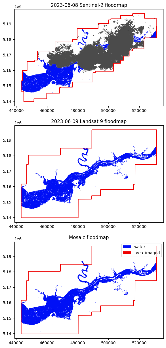
Step 12: Join the floodmaps of Sentinel-2 and Landsat#
Here we join the floodmaps of the two satellites using the max mode.
warnings.filterwarnings('ignore')

area_imaged = post_flood_shape_l9.loc[post_flood_shape_l9['class'] =='area_imaged']

# Remove flood traces for the max extent join
post_flood_shape_l9 = post_flood_shape_l9.loc[post_flood_shape_l9['class'] !='flood_trace']
post_flood_shape = postflood_shape.loc[postflood_shape['class'] !='flood_trace']

postflood_mosaic = postprocess.mosaic_floodmaps([post_flood_shape, post_flood_shape_l9], area_imaged.geometry.values[0], mode = 'max',
                                                classes_water=['water','flood_trace'])
fig, ax = plt.subplots(3, 1, figsize=(20, 15))
plot_utils.plot_floodmap(post_flood_shape, ax=ax[0], legend = False)
ax[0].set_title(f"{date_post} Sentinel-2 floodmap")
plot_utils.plot_floodmap(post_flood_shape_l9, ax=ax[1], legend = False)
ax[1].set_title(f"2023-06-09 Landsat 9 floodmap")
plot_utils.plot_floodmap(postflood_mosaic,ax = ax[2], legend = True)
ax[2].set_title(f"Mosaic floodmap")
Text(0.5, 1.0, 'Mosaic floodmap')
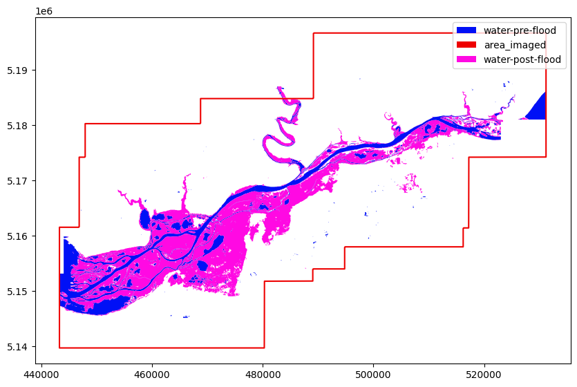
prepost_shape_final = postprocess.compute_pre_post_flood_water(postflood_mosaic, preflood_shape)
prepost_shape_final = prepost_shape_final.loc[prepost_shape_final['class'].isin(['water-pre-flood','water-post-flood','area_imaged'])]
plot_utils.plot_floodmap(prepost_shape_final)
<Axes: >
Licence#
The ML4Floods package is published under a GNU Lesser GPL v3 licence
The WorldFloods database and all pre-trained models are released under a Creative Commons non-commercial licence. For using the models in comercial pipelines written consent by the authors must be provided.
The Ml4Floods notebooks and docs are released under a Creative Commons non-commercial licence.
If you find this work useful please cite:
@article{portales-julia_global_2023,
	title = {Global flood extent segmentation in optical satellite images},
	volume = {13},
	issn = {2045-2322},
	doi = {10.1038/s41598-023-47595-7},
	number = {1},
	urldate = {2023-11-30},
	journal = {Scientific Reports},
	author = {Portalés-Julià, Enrique and Mateo-García, Gonzalo and Purcell, Cormac and Gómez-Chova, Luis},
	month = nov,
	year = {2023},
	pages = {20316},
}
Acknowledgments#
This research has been supported by the DEEPCLOUD project (PID2019-109026RB-I00) funded by the Spanish Ministry of Science and Innovation (MCIN/AEI/10.13039/501100011033) and the European Union (NextGenerationEU).
 funded by MCIN/AEI/10.13039/501100011033.")